Critical power is, theoretically, the work output that one can sustain indefinitely. The concept is that an individual will, after sustained maximal effort work, reach a point at which their aerobic energy systems match the demands placed on the muscle. Although there is some validity to the model, it remains idealistic and is contested in the literature.
The critical power model was initially proposed and assessed using individual muscles. Soon thereafter, the model was adopted by cyclists and adapted by swimmers and runners. Traditional testing, regardless of exercise modality, is for an athlete to perform several maximal-effort time trials. The results are plotted and a regression is fit to the data. The results are either a linear or hyperbolic function and can return an athlete’s critical power, their anaerobic energy capacity, and theoretical max speed. For example, the two-parameter model returns approximations of an athlete’s critical power (CP) and anaerobic energy reserve (W’). Conversely, the exponential decay model is empirical, and the values returned are hypothesized to represent various physiological metrics. Researchers are, typically, more interested in physiologically-rooted models because they are meant to represent phenomena that occur within the muscle.
By testing an athlete over various durations, researchers can plot the athlete’s power-duration curve. The power-duration curve describes an athlete’s theoretical maximal effort that can be sustained for a given duration or time. A result of the parabola is the ability to estimate an athlete’s capacity for any duration, eliminating the need for more time trials. Subsequently, by tracking a racer’s results, the power-duration curve can be updated to reflect improvements and decrements in their abilities.
Apply the Critical Power model to your training programs with Training and Racing with a Power Meter
Sign-up for a free preview of the book You can unsubscribe anytime. For more details, please see our Privacy Policy.
You should receive an email shortly with a link to preview Training and Racing with a Power Meter
Several drawbacks exist regarding the critical power model. Primarily, researcher have argued that physiologically rooted models coincidentally coincide with metrics like critical power. This is because model parameters are fitted to minimize residual error. Therefore, the parameters should still be regarded as being empirical. Moreover, the models are constrained because they are limited in their ability to consider fatiguing factors beyond those in the muscle. For example, the two-parameter model was validated for durations between two and thirty minutes. During the first two minutes, the body is responding to the exercise demands. Since there is a delay, muscles are disproportionately reliant on anaerobic energy stores. One can envision this as there being a ramp increase in critical power until the steady-state is reached. When athletes surpass the 30-minute mark, fatigue develops locally and systemically. Although the model accounts for local, or muscular, fatigue accumulation, it cannot account for systemic factors that are beyond the muscle. Systemic fatigue accrued due to cardiovascular adjustment that stem from, for example, dehydration or decreases in central drive due to perceptual factors like pain cannot properly be modelled.
Several models have attempted to expand and improve on the two-parameter model. The three-parameter and exponential models introduces a maximal-power (Pmax) parameter. In doing so, these models include a y-intercept which shifts the parabola left while still modelling the athlete’s critical power. These models were still limited in their ability to model critical power beyond thirty minutes.
Recently, the OmniDomain Power Duration model was developed to extend the two, three, and exponential critical power models beyond the thirty minute threshold. The researchers utilized Peronnet and Thibault’s previous work on Maximal Aerobic Power (latter portion of the model) which includes a decay function. This concept was utilized to model the decline in critical power with increasing duration.
With the adoption of fitness tracking and positional tracking devices, the critical power model can be adapted for runners and swimmers. The approach when testing critical velocity (CV) remains the same as it does for critical power. The only difference is that velocity can be substituted for power which results in the critical velocity model with the parameters being max distance travelled above critical velocity (D’) and maximal speed (Vmax).
Modelling Critical Velocity
Apart from the inverse model, critical velocity models are parabolic. The inverse model is a linear regression that can be achieved using the lm() function. Alternatively, fitting a non-linear regression in R is achieved using the nls() function. Both functions are native to R and do not rely on users installing external packages.
Unlike the lm() function, nls() tasks users with setting initial parameter values. The function then optimizes the parameters to minimize residual errors. Subsequently, the starting values are consistently applied for all of the models such that critical velocity is 4 m/s, maximal speed is 9 m/s, and D’ is 150 m.
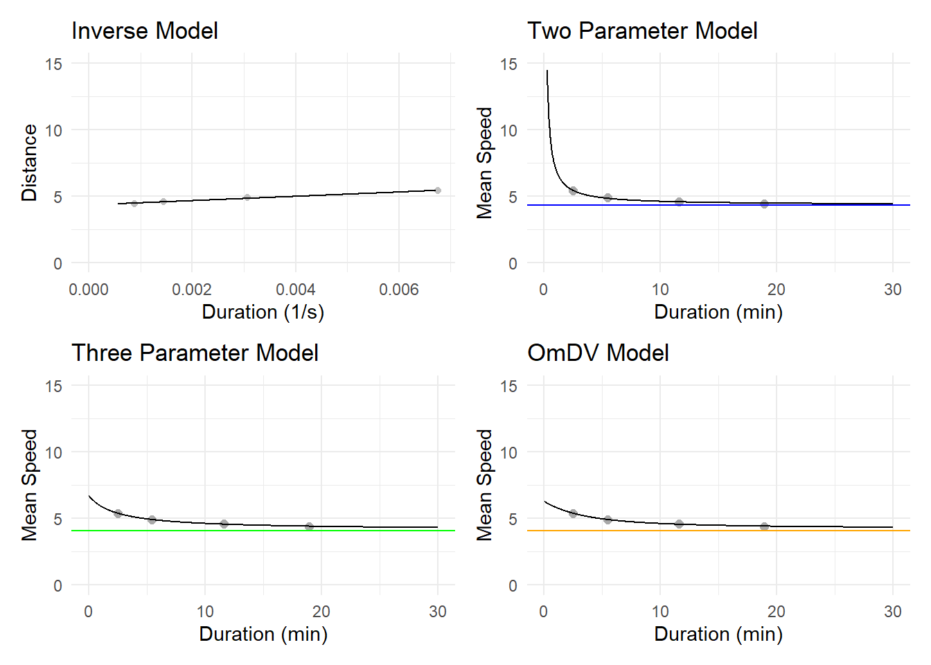
Below, critical velocity is modelled using the inverse, two parameter, three parameter, and OmniDomain velocity duration models. Seeing that the time trials do not extend beyond 30 minutes, the extended function within the OmVD model trends to zero. Therefore, the simple OmVD model will be utilized.
Below is a runner’s hypothetical time trial results. They completed four time trials over the course of two weeks, and ensured that fatigue accrued from previous sessions did not impact time trial performance.
# since the data is simulated, nls() needs controls in place so that it doesn't return a warning or error omvd.formula <-"mean.speed ~ crit.speed + d.prime * (1 - exp(-1 * duration * (max.speed - crit.speed)/ d.prime))/ duration"omvd <-nls(omvd.formula, data = time.trials, start =c(crit.speed =4, d.prime =150, max.speed =9),control =nls.control(warnOnly =TRUE, minFactor =1e-5, tol =1e-10), algorithm ="port", lower =c(2, 100, 5,8))
Critical speed can be modeled using the models outlined above. The models return similar critical speed values and maximal speed. Anaerobic capacity, D’, ranges from 162.5 m to 371.1 m, which is a realistic range. Unfortunately, since D’ is highly variable, the utilization of the critical speed models are limited in their ability to predict race outcomes.
Parameters from the inverse and two parameter models are the same because the inverse model is derived from the two parameter model. Both models were included in the analyses to illustrate the various methods of modeling critical speed. Maximal speed returned from the three parameter and OmVD models are similar. The values returned are nearer to an individual’s maximal aerobic speed than a realistic maximal speed. This is probably a symptom of the data being simulated and can be addressed in the future.
Subsequent analyses can explore how testing modalities affect the model fit. Moreover, with the popularity of positional tracking data, various methods of estimating critical speed have recently emerged and can be utilized in future work.
References
Drake, Jonah & Finke, Axel & Ferguson, Richard. (2022). Modelling human endurance: Power laws vs critical power. 10.1101/2022.08.31.506028.
Puchowicz, M. J., Baker, J., & Clarke, D. C. (2020). Development and field validation of an omni-domain power-duration model. Journal of sports sciences, 38(7), 801–813. https://doi.org/10.1080/02640414.2020.1735609
Roecker, K., Mahler, H., Heyde, C., Röll, M., & Gollhofer, A. (2017). The relationship between movement speed and duration during soccer matches. PloS one, 12(7), e0181781. https://doi.org/10.1371/journal.pone.0181781
Apply the Critical Power model to your training programs with Training and Racing with a Power Meter
Sign-up for a free preview of the book You can unsubscribe anytime. For more details, please see our Privacy Policy.
You should receive an email shortly with a link to preview Training and Racing with a Power Meter